Xenium spatial transcriptomics

About the dataset

The example dataset is the 10x Genomics Xenium Mouse Brain Coronal Section, distributed by the SpatialData project as a Python-compatible OME-Zarr store. It contains:

• ~5 million transcripts (points/transcripts)
• Cell boundary polygons (shapes/cell_boundaries) and nucleus boundaries
• 4-channel fluorescence tissue image (images/morphology_focus)
• H&E image (images/he_image)
• Cell segmentation label mask (labels/cell_labels)

Download

Download the Xenium example store from the SpatialData datasets page. The store is a directory named xenium_ex.zarr; place it wherever is convenient (the path below is arbitrary):

# Adjust path to wherever you downloaded the store
xenium_path = "/path/to/xenium_ex.zarr"

Load and inspect

using SpatialOmics

xen = read(SpatialDataZarr(), xenium_path)

# Element inventory
keys(elements(xen))

# Coordinate systems
coord_systems(xen)

# Top 20 expressed genes
tx = points(xen, "transcripts")
top_features(tx, 20)

# Cells with transcript counts
counts = count_per_instance(tx)
sort(collect(values(counts)); rev=true)[1:10]   # top 10 cells by count

Visualise

A subsampled scatter over the full slide gives a quick overview of tissue layout and transcript distribution.

using CairoMakie

fig = Figure(size=(900, 900))
ax  = Axis(fig[1, 1]; aspect=DataAspect(), yreversed=true,
           title="Xenium — transcript overview")

n   = length(coords(tx))
idx = sort(rand(1:n, 200_000))   # subsample for speed
scatter!(ax, coords(tx)[idx]; markersize=0.3, color=(:black, 0.08))
tightlimits!(ax)
fig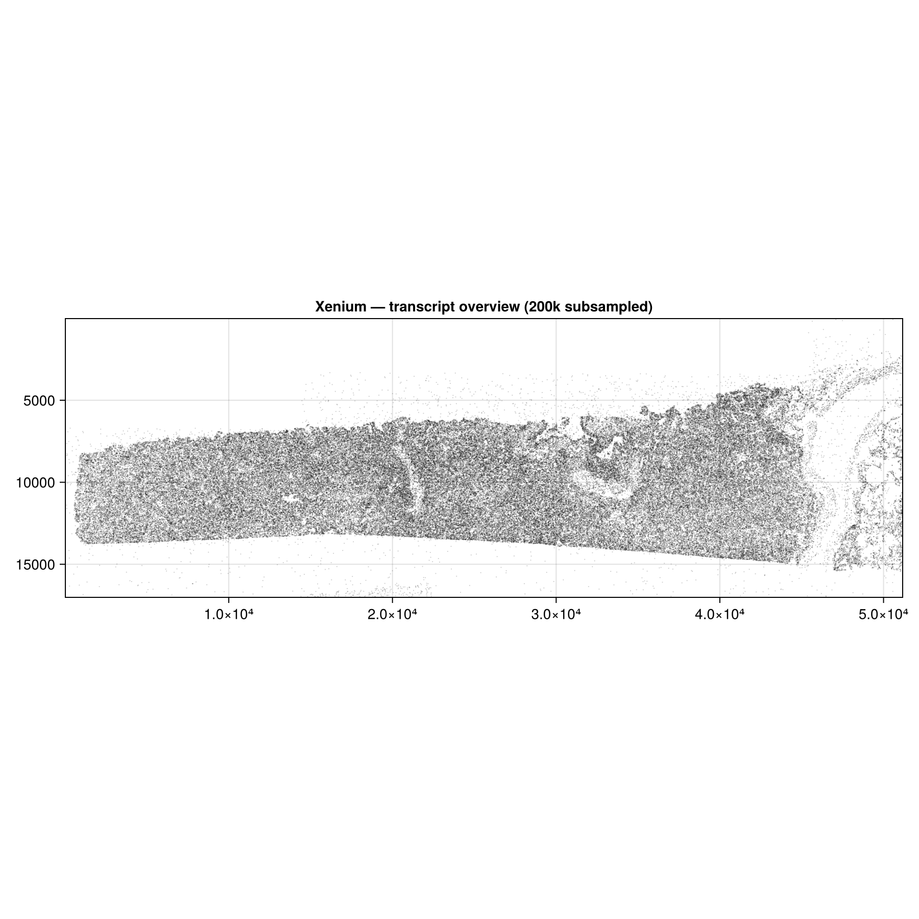

Explore a region of interest

Define a spatial extent and build a lazy view. Each plot verb applies the filter independently — no intermediate copies are made.

ext = SpatialExtent(3500.0, 3700.0, 2800.0, 3000.0; coord_system="global")
roi = view(xen, ext)

fig = Figure(size=(600, 600))
ax  = Axis(fig[1, 1]; aspect=DataAspect(), yreversed=true,
           xlabel="x (µm)", ylabel="y (µm)")

image!(ax,   scaleminmax(channel(images(roi, "morphology_focus"), 1)))
poly!(ax,    shapes(roi, "cell_boundaries");  color=:transparent,
                                              strokecolor=:cyan, strokewidth=0.5)
scatter!(ax, points(roi, "transcripts");      markersize=1.5, color=(:red, 0.4))
tightlimits!(ax)
fig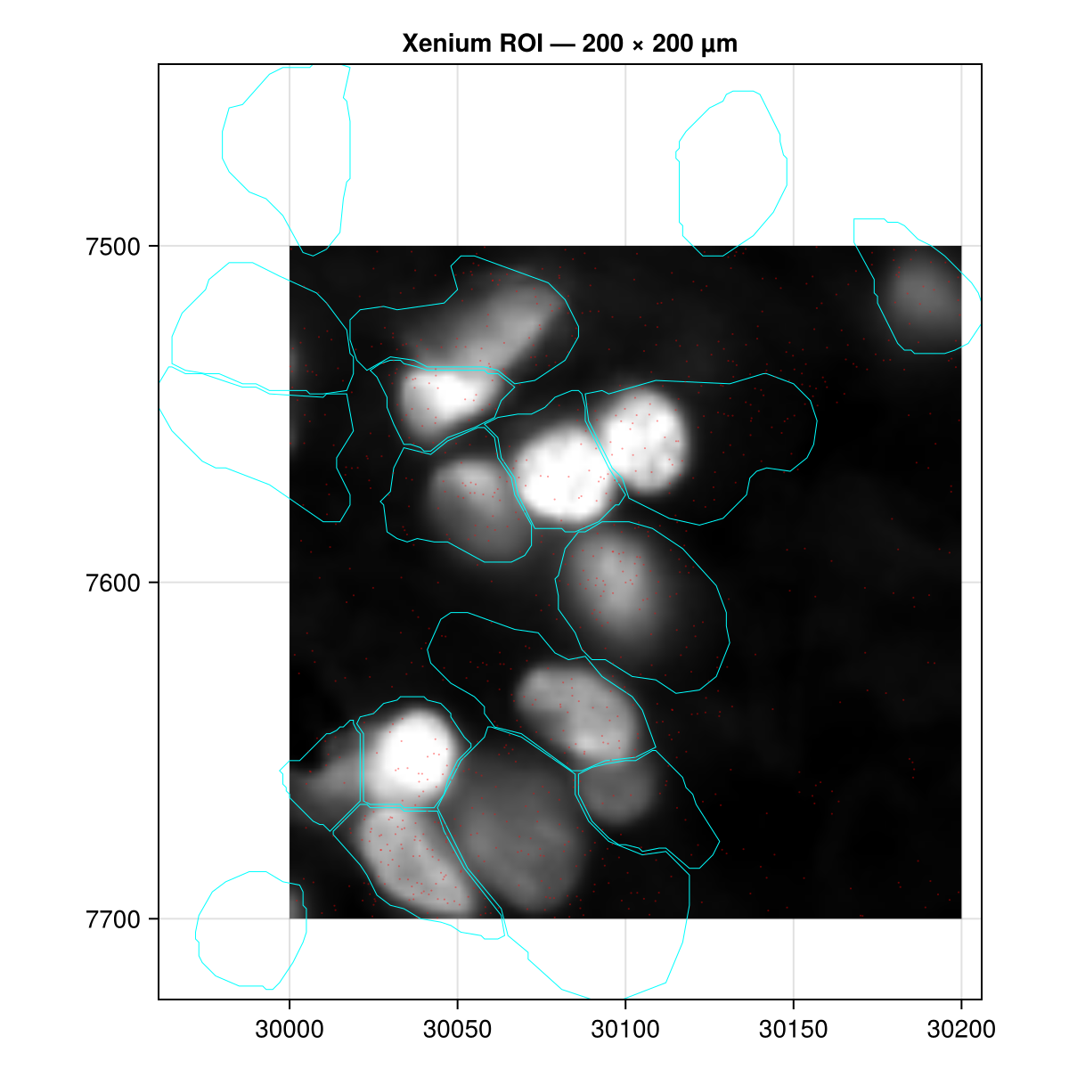

Creating a subset

The committed test fixture at test/data/xenium_small.zarr was created from a 200 µm × 200 µm region of this dataset. The test/make_fixtures.jl script automates this in two passes:

Pass 1 — generate overview figure and pick coordinates:

# Run: julia --project=. test/make_fixtures.jl
# Inspect docs/src/assets/xenium_overview.png
# Fill in XEN_XMIN / XEN_XMAX / XEN_YMIN / XEN_YMAX in the script

Pass 2 — create the fixture:

# After filling in coordinates, re-run the script:
# julia --project=. test/make_fixtures.jl
# This writes test/data/xenium_small.zarr and docs/src/assets/xenium_roi.png

Internally the script uses:

ext = SpatialExtent(XMIN, XMAX, YMIN, YMAX; coord_system="global")
roi = view(xen, ext)

sub = SpatialDataset()
sub["transcripts"]     = collect(points(roi, "transcripts"))
sub["cell_boundaries"] = collect(shapes(roi, "cell_boundaries"))
sub["morphology_focus"] = images(roi, "morphology_focus")

write!(sub, "test/data/xenium_small.zarr", SpatialDataZarr())

view is lazy — no data is read until collect or the plot verb materialises it. The resulting zarr is in SpatialOmics' native format and is loaded directly by read(SpatialDataZarr(), path) without the full dataset.

Working with the committed fixture

The fixture is small enough to use in offline development and CI:

ds = read(SpatialDataZarr(), joinpath(pkgdir(SpatialOmics), "test", "data", "xenium_small.zarr"))

tx  = points(ds, "transcripts")
shp = shapes(ds, "cell_boundaries")
img = images(ds, "morphology_focus")

@show length(coords(tx))
@show nchannels(img), channel_names(img)
@show top_features(tx, 5)